Introduction
In the past two posts, I introduced logarithms and the log-normal distribution—key concepts in investment analysis—and explained why taking the log of a ratio isn’t literally a return but a measure of investment duration.
- [Intermediate 34] Logarithms and log scales in investing — why use logs [Korean]
- [Intermediate 35] Log-normal distribution — why it matters in finance [Korean]
In investment analysis, the natural logarithm of the price ratio (the log return) is also known as the continuously compounded return, the time derivative of log price, or the rate of return on log price. This post explores why log return reflects time rather than return, yet can still be validly treated as a return measure.
Note: This article is an English translation of the following Korean post with the help of ChatGPT: [Intermediate 36] What Is the Essence of Log Return? (Why It’s Not Technically a Return—Yet Can Be Treated as One?)

⚠️ Note: This post does not recommend any product or strategy. All figures represent past observations, not forecasts. Results may vary depending on data, period, or methodology, and there may be errors in data processing. Verbs are used in the present for convenience, but all descriptions refer to past analysis.
1. Why Log Returns Represent Time
Consider an asset growing at a continuous compound rate \(r\) over time \(x\). Its price ratio becomes:
$$ y = {(1 + r)}^x $$
Taking the natural log yields:
$$ \ln(y) = \ln{(1 + r)}^x = x \ln{(1 + r)} $$
Here, \(\ln(y)\) is the log return. Since \(\ln(1 + r)\) is constant, \(\ln(y)\) scales linearly with time \(x\). Thus, log return is essentially a measure of time. It quantifies how many compounding periods are needed to achieve a factor of \(1 + r\).
When plotted on a log scale, this becomes visually clear:
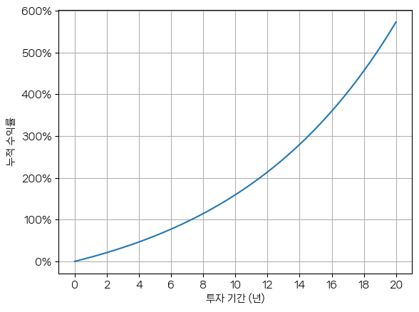
- On a linear scale, compound growth accelerates exponentially.
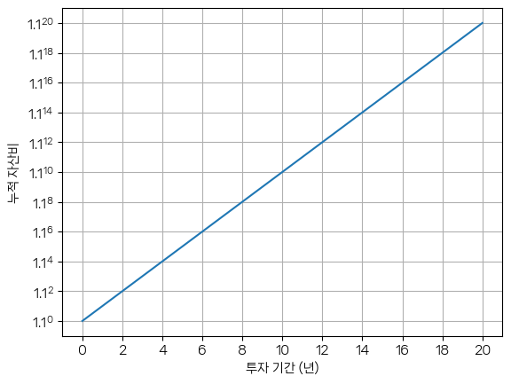
- On a log scale, it appears as a straight line, because:
$$ y = \log_{1.1}({1.1}^x) = x $$
Even if you change the logarithm base, the line remains linear—only the slope changes. Taking the natural log gives:
$$ y = \ln({1.1}^x) = x \ln(1.1) $$
So \(\ln(1.1) \approx 0.095\) becomes the slope.
Moreover, because log return is time, compound growth (multiplication) transforms into addition:
e.g., doubling each year for 3 years:
$$ 2^1 \times 2^2 = 2^3 = 8 $$
On a log base‑2 scale:
$$ \log_2{(2^1 \times 2^2)} = \log_2{2^1} + \log_2{2^2} = 1 + 2 = 3 $$
This additive property underlies the usefulness of log returns.
2. Why Treat Log Returns as “Returns”
Why use the natural log \(e\)? Because near zero, \(\ln{(1 + x)} \approx x\).
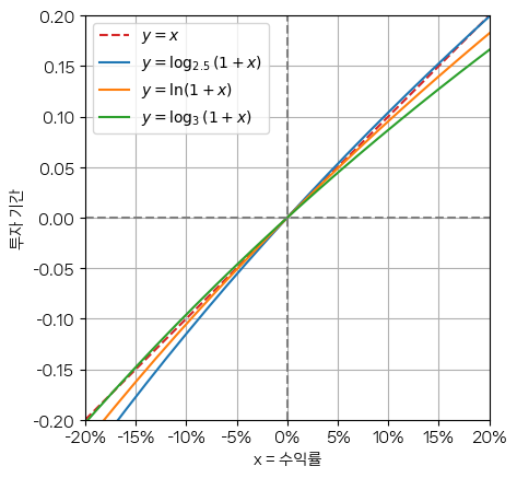
Graphing log bases 2.5, \(e\), and 3 against the line \(y = x\) shows that for returns in [−20%,20%], natural-log-based returns align best with linear returns.
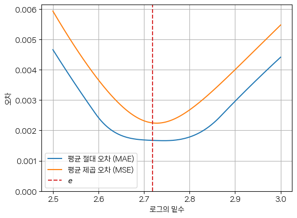
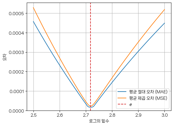
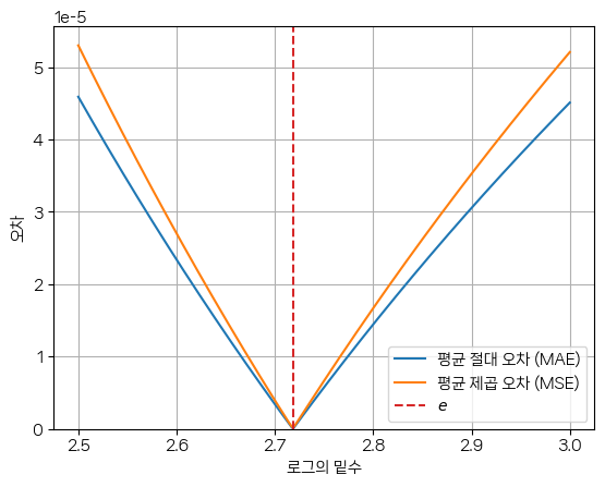
In narrower ranges like [−1%,1%], \(e\) remains the closest match. Hence, log returns approximate actual returns when returns are small, while still preserving additive compounding.
3. The Meaning Behind the Log-Return Formula
The log-return formula stems from continuous compounding:
$$ \lim_{n \rightarrow \infty}{(1 + r/n)}^n = e^r $$
Letting \(y = e^r\), we get:
$$ \ln(y) = r $$
At first glance, this suggests log return equals simple return \(r\), which seems contradictory. As previously discussed, log return is time—closely approximating return only around \(r \approx 0\), where:
$$\lim_{r \rightarrow 0}\frac{ \ln{ (1 +r) }} {r} = 1$$
Generalizing, for base \(s\), you find that only with \(s = e\) does \(\lim_{r \rightarrow 0}{\frac{ \log_s{ (1 + r) }} {r}} = 1\), reinforcing why \(e\) is fundamental in log returns.
Conclusion
We have shown that log return inherently measures time, not simple return. Yet, because in small-return ranges \(\ln(1 + x) \approx x\), we can use log returns as practical proxies. The natural logarithm’s base \(e\) emerges naturally as the unique choice that best aligns log return with actual return in continuous-time finance.
In my view, the formulas commonly used to explain and derive log returns lack rigor. The way the formulas are defined and developed does not quite align with the purpose for which they are being used.
'주식투자' 카테고리의 다른 글
| [중급 부록 A3] 이 커버드콜 ETF의 기초자산은 무엇일까? (피어슨 상관 계수를 이용한 닮은 ETF 찾기 2) (0) | 2025.07.12 |
|---|---|
| [중급 부록 A2] 이 자산은 무엇과 비슷했을까? (피어슨 상관 계수를 이용한 닮은 ETF 찾기) (0) | 2025.07.11 |
| [중급 부록 A1] 피어슨 상관 계수의 기하학적 해석 (표준화한 두 자산 간의 선형 상관성) (0) | 2025.07.11 |
| 해외증권세전합병입금 (상장 폐지로 인한 매도 대금, 한국투자증권 미니스탁) (0) | 2025.07.01 |
| [중급 48] 투자에서 분석과 예측의 역할은 무엇일까? (퀀트 투자는 주관적 판단이 배제된 투자일까?) (0) | 2025.06.29 |
| [중급 47] 통계량은 왜 예측이 아닌가? (분석 기간에 따른 검정 결과의 변화 사례) (0) | 2025.06.28 |
| [중급 46] 통계적 검정은 어떤 원리일까? (대응 표본 t-검정; paired t-test) - 검정은 미래를 예측하는 분석이 아니다 (0) | 2025.06.27 |
| [중급 45] 투자 전략 비교의 신뢰성 평가는 신뢰할 수 있는 것일까? (0) | 2025.06.26 |


